Lecture 8: Large Language Models (LLMs)
Deep Unsupervised Learning - Berkeley - Spring 2024
This page covers Lecture 8 from the Deep Unsupervised Learning (DUL) course, Berkeley Spring 2024.
Key Details:
- Topic: Large Language Models (LLMs)
- Instructor: Hao Liu, Final-Year Ph.D. student at Berkeley
- Status: These notes are currently a work in progress. The lecture is packed with detailed insights, and additional content will be added soon.
- Outline: Lecture split into 2 sections ( basics, scaling laws and capabilities ) and 2nd section for practical guidelines for research and practical purposes.
Stay tuned for updates as I continue to expand and refine these notes to capture the full depth of the lecture!
Language Model Abstraction:
-
A Language Model is a probability distribution over sequences:
- Likelihood distribution:
- Uses sequence of tokens
- Parameters
-
Typically Language Models are autoregressive since it factorize sequences auto regressively.
- Formula:
-
T (tokens) going to condition on only tokens before it, Models are parameterized by a transformer.
-
So in summary the model is an autoregressive likelihood distribution over a sequence of tokens.
-
Autoregressive Factorization, despite the other different ways to model language sequences, is done for:
- Every Bit becomes part of the supervision, predicting every token and the tokens become prediction targets.
- Next Token Prediction
- It turned out to be crucial for the scaling of the language model.
- Natural for Conversational AI.
- Models suitable for following up conversation by Predicting Future Tokens.
- Every Bit becomes part of the supervision, predicting every token and the tokens become prediction targets.
-
Maximum Likelihood (Modeling Likelihood):
- The Goal is to make the observed data likely predictable under the model.
- The Objective Function Formula:
- D is for example 1.5 Trillion Tokens in Llama.
- is for example 7 to 70 billion parameters.
- The Objective Function Formula:
- The Goal is to make the observed data likely predictable under the model.
Language Model Training:
Stages Of Learning
- Pretraining:
- Done in Large scale.
- Unsupervised Learning.
- Maximizing Likelihood over a Very Large dataset of sequences.
- Finetuning:
- Model Specializing stage.
- Focusing on specific set of tasks.
- Learning from feedback:
-
Improving the model by giving feedback.
-
Focusing on outputs feedbacks such as human feedback in RLHF and debug messages or other methods like DPO.
-
The model is generally good and better on the fine-tuned task, but it needs to comprehend and follow user’s intention so it needs users’ feedback, and this stage focuses on how to use human feedback to align the model outputs with user desired outputs.
-
The Lecture focuses mostly on Pretraining LLMs and then will pass by some fine-tuning and learning from feedback.
- Because Most of the time, basically pretraining stage determines how good the model you built is.
The reason behind choosing Unsupervised Learning :
-
Because of the richness in unsupervised data (unlabeled data) sources.
-
Better Generalization in most of the tasks as the model captures the distribution better.
- it’s shown better results than supervised learning in literature.
-
For example, from the Llama paper the pretraining stage:
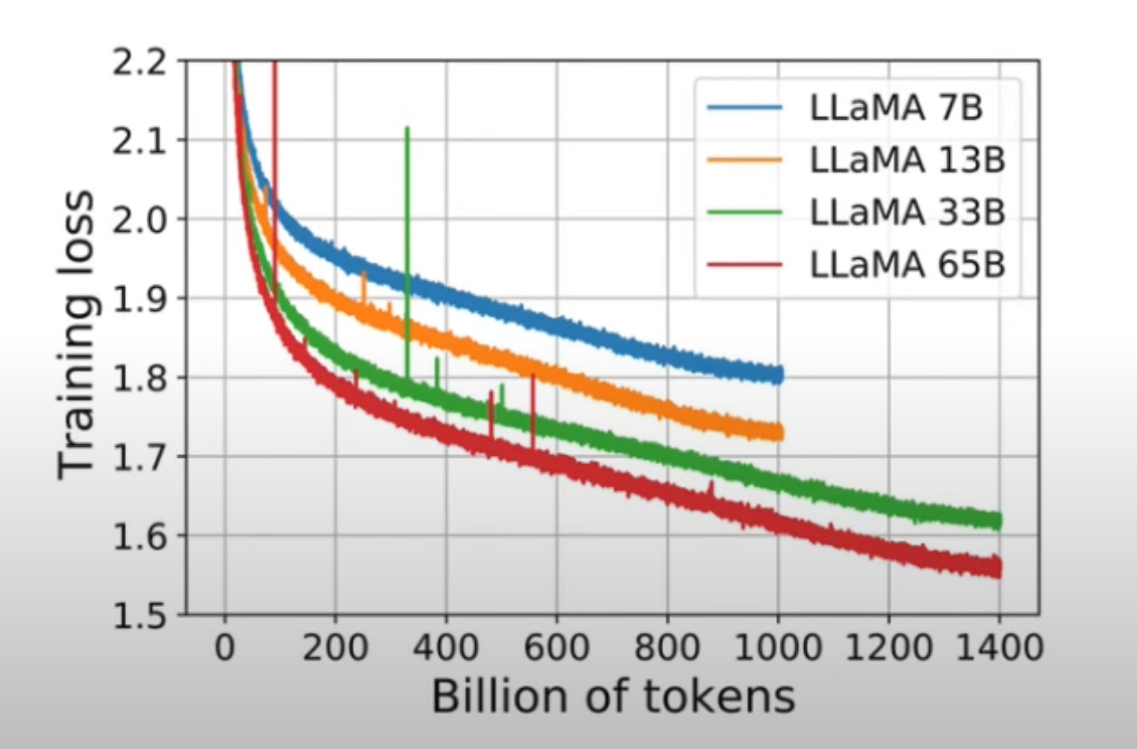
- Y-axis: The Average most Likelihood Loss (Lower is better)
- X-axis: Number of Tokens seen during training stage.
- Notice that the curves aren’t saturated and are continuously decreasing.
- We still have way more available data on the internet for language learning.
Scaling Compute
“The biggest lesson that can be read from 70 years of AI research is that general methods that leverage computation are ultimately the most effective, and by a large margin.” — The Bitter Lesson, Richard Sutton, 2019
- In summary: The major AI successes is going to come from methods that leverage computation
- Typically the goal is to model the data distribution better by adding more compute.
- Compute analogy
- It’s the forward and backward pass (back-propagation).
- Mostly spent on matrix multiplications (matmul)
- Measured using (FLOPs)
- As MatMuls are basically doing floating points multiplications and additions.
- Compute Cost Estimating Formula:
- N: Number of parameters, basically (model) size.
- D: (data) size.
- s: context size.
- d: (hidden) dimension, the size projection dimension.
- It turned out that size matters, lol.
- TL;DR Using more tokens (larger dataset), larger context windows (longer sequences of data), and larger models add up compute costs.
- Does that mean AGI will require the electricity of a country’s households ?
Tokens:
- Byte-Based Tokenization :
- Most Generic for all types of data sequences.
- It’s too long, leading to a lot more compute cost.
- little bit unnecessary in some perspectives.
- Character-Based Tokenization :
- Similar problem as Byte-Based long words require too many tokens.
- Word-Based Tokenization :
- Some words will share similar semantic meaning but different tokenization.
- cat and cats should have the same semantic meaning. (Sorry, am a cat 😸 guy)
- Some words will share similar semantic meaning but different tokenization.
- Sub-word-Based Tokenization :
- A trade-off in between both worlds.
- Byte-Pair Encoding: Replacing top appearing pairs with a new token.
- It has the heart of frequency based feature extraction algorithm in classical classification problems.
- Example: tiktoken (used by OpenAI models like GPT-4).
- Pros:
- Compact Vocabulary: Byte-based tokenization drastically reduces the vocabulary size since all tokens can be built from a limited set of byte sequences.
- Multilingual Support: It handles characters from any language (e.g., Chinese, Arabic, emojis) without requiring separate tokenization logic.
- Consistency: Byte-level tokenization avoids ambiguity in how characters or sequences are split.
- Allows handling diverse character sets, including non-ASCII characters, without special preprocessing.
- Avoids complications arising from Unicode normalization. Each character or emoji is consistently tokenized regardless of its codepoint.
- Repeating until having a dictionary for tokens and a vocab size of tokens
In 2017, researchers tried training LSTM with more compute on sentiment analysis on amazon reviews, where it learns a sentiment neuron (+positive / -negative) after training to predict the next word on a large dataset of Amazon reviews.
-
They basically did autoregressive next token prediction.
-
The following graphs helped them deduce that:
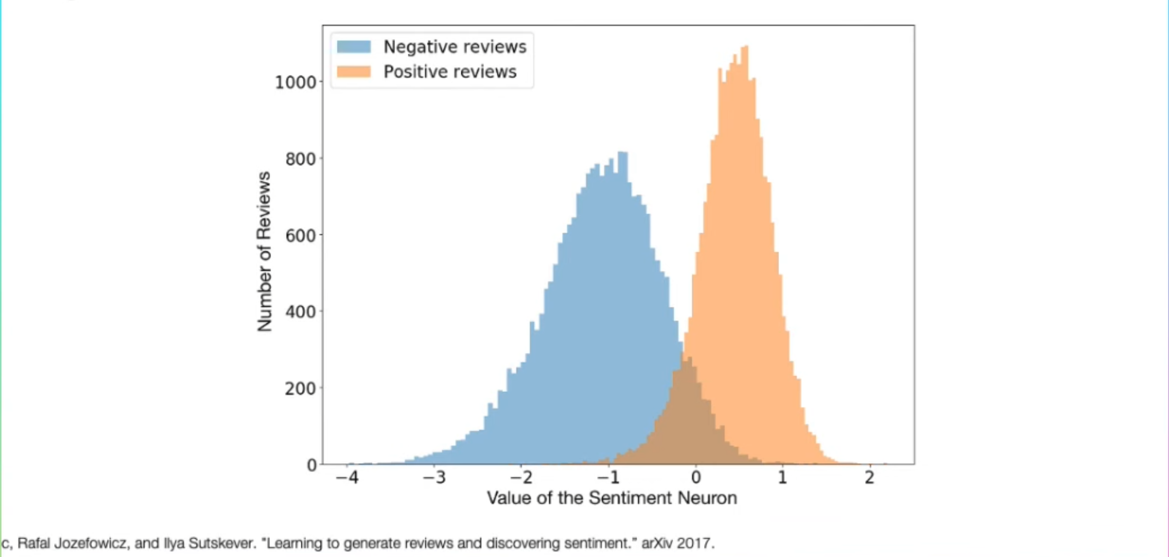
- X-axis Observations:
- There are some neurons can be used to control the output of the LSTM.
- Y-axis Observations:
- Number of LSTM’s output that’re either (positive) or (negative).
- By controlling the values of certain neurons, you can influence the LSTM’s generative output to generate either (positive) sentiment or (negative) sentiment in reviews.
- what a scary observation for product review batting 👾💀.
- X-axis Observations:
-
The model was able to comprehend human sentiment (positive / negative) by benefitting from more compute, that was a difficult language task back 7 years ago.
-
Visual heatmap of sentiment neurons’ values was generated on top of a document composed of 6 random highly contrasted IMDB reviews:
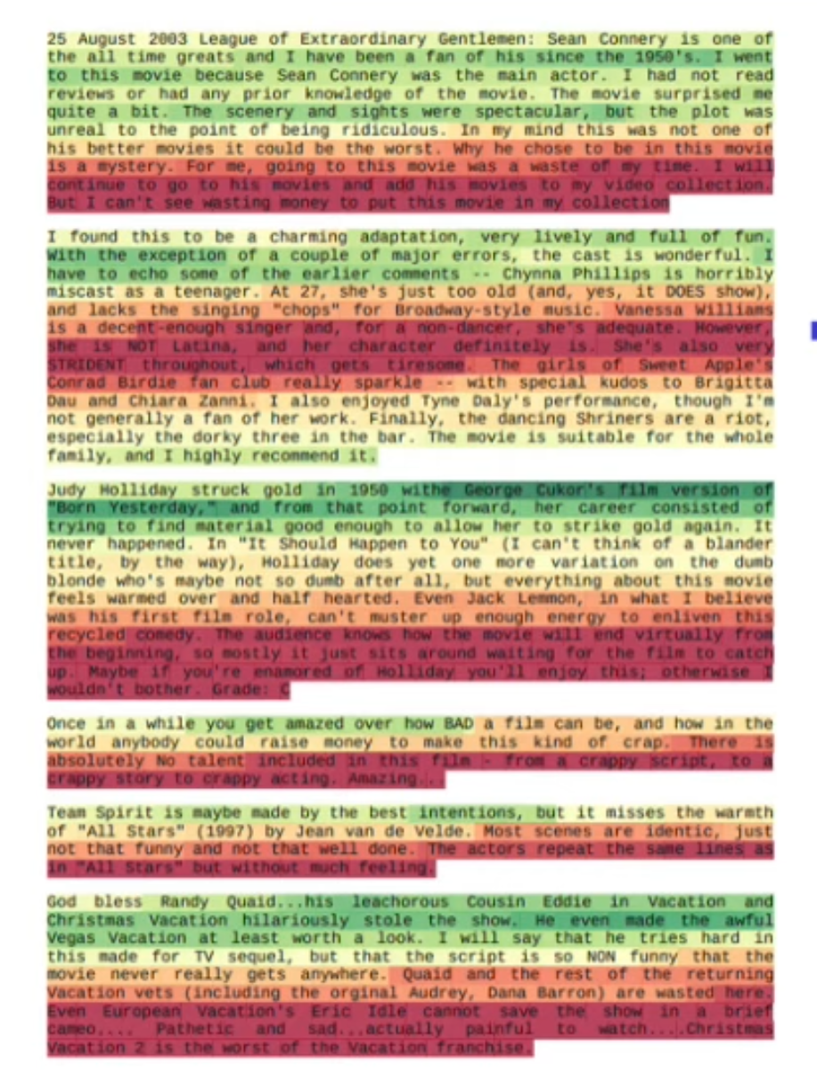
- Red for (negative) and Green for (positive) that was an advancement back in 2017.
Then came a new proposed architecture called Attention, which scales much better than LSTMs.Transformer models asymptotically outperformed LSTMs because of better use of context and specially when context window increases.
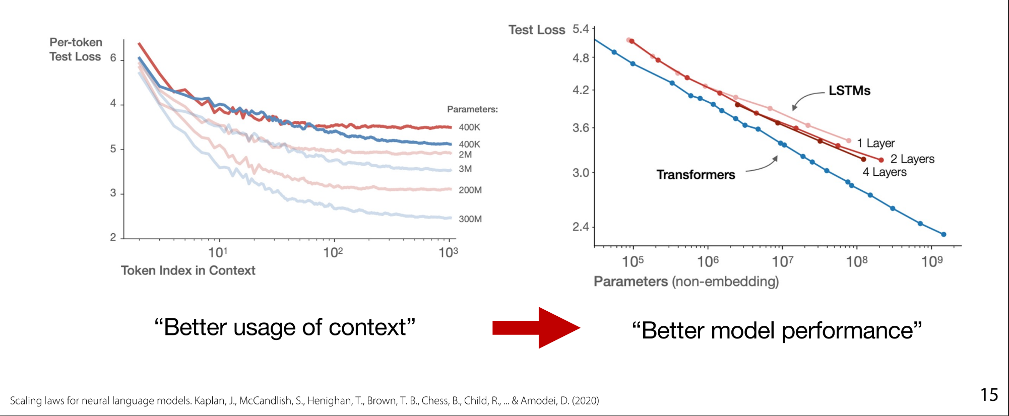
- Red-Lines for LSTMs, while Blue ones beating the up LSTMs are Transformers.
- Left Figure shows per token test-loss:
- Looking at a particular position over the 1000 tokens which model predicts that particular token better.
- X-axis: the token index.
- Y-axis: Loss corresponding to that particular token.
- Right Figure shows per model size (number of parameters) test-loss:
- Transformers measured parameters excluded embedding parameters.
- The bigger the model, the bigger the gap between the 2 models performance.
- Which’s obviously because of the wiser usage of context using attention mechanism.
- X-axis: Parameters number - model size.
- Y-axis: Loss corresponding to specific model size
- By scaling-up model size Transformers show pretty linear scaling, while LSTMs saturate early.
- Attention helps keeping focus and information on past tokens without forgetting them.
- LSTM you had to maintain certain hidden states, but in attention you can directly attend to any past token, the model doesn’t have this information bottleneck.
- You can easily increase model parameters by adding bigger MLP networks (Big FFNs, highly scalable)
- which are large matrix multiplications so it scales well with modern GPUs and TPUs.
Pretraining Objectives
We talked about full autoregressive prediction objective used by models like GPT, LLaMA. However, there are other objectives that define the training of the model, for example:
-
Masked Token Prediction used by: BERT, ELMO.
-
Prefix autoregressive prediction used by: T5.

-
Masked token prediction is an effective objective for masked language models, as it helps them learn the full semantic meaning of a sequence.
- Example: Embedding Model for search, retrieval, catching semantic meaning better.
-
Prefix autoregressive predictions are an interesting alternative to masked token prediction for PLMs, but they are not yet widely used.
- Most of Encoder-Decoder models they can be reformulated as autoregressive prediction but with a different attention mask like a prefix mask, the Encoder is the bidirectional attentive while the autoregressive part is the decoder, Encoder is usually bi-directional (Masked), the auto-regressive one is the decoder.
-
For visualization and clarification:
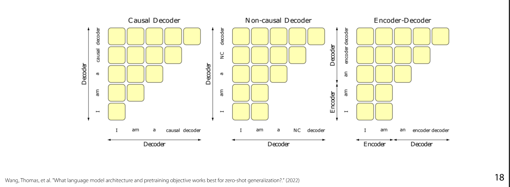
- X-axis and Y-axis are both the sequence of tokens.
- PLM (Prefix Language Model) is the Non-Causal Decoder Middle graph.
- Full Autoregressive widely used GPT model is the Causal Decoder first graph.
- Different Objects but approximately similar amount of FLOPs computationally.
- The Last one, which is the Encoder-Decoder Transformers tends to out to be the most scalable.
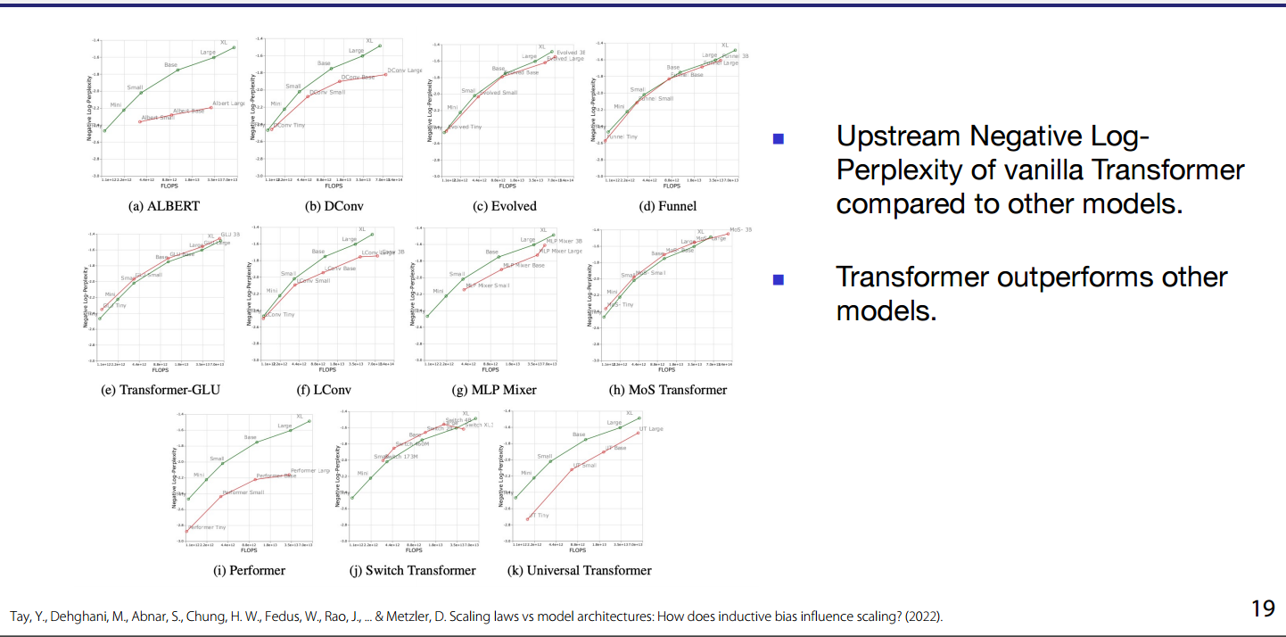
- Upstream (negative) Log-perplexity : Vanilla Transformer outperforms other models.
- Downstream accuracy : Vanilla Transformer outperforms other models.
- An interesting question to explore is how the performance of the vanilla model compares to that of other derived models in terms of FLOP efficiency/costs.
-
Researchers tried out interesting ideas and modifications on Transformers architecture, so when you do research remember to check scalability against flops vs. Vanilla.

LLM-Compute Costs
- Hidden size of (MLP) is usually 4d because of expanding factor of MLP network.
- Llama (s << 6d), so approximately
- Empirical performance of model has power-law relationship with each factor:
-
log-log correlation between factors.
-
-
-
as , allocate more compute to parameters (a), or tokens (b)
-
Researchers tried training different model sizes / number of tokens to conclude a scaling hypothesis
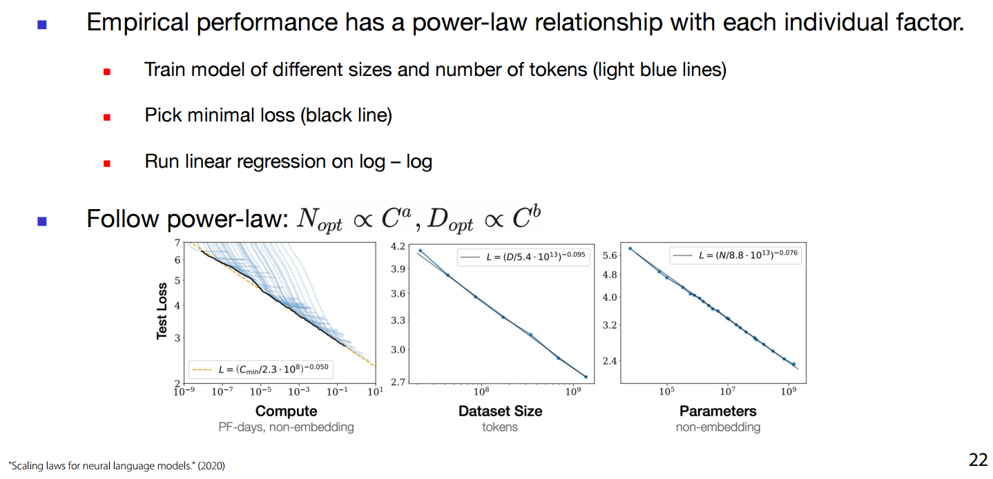
- Different compute allocations on x-axis.
- Test Loss on un-seen data on y-axis.
- The lowest point for each particular configuration (Compute Allocation), the black line- shows a log-log correlation.
-
which to choose a (more compute to parameters) or b(more compute to tokens):
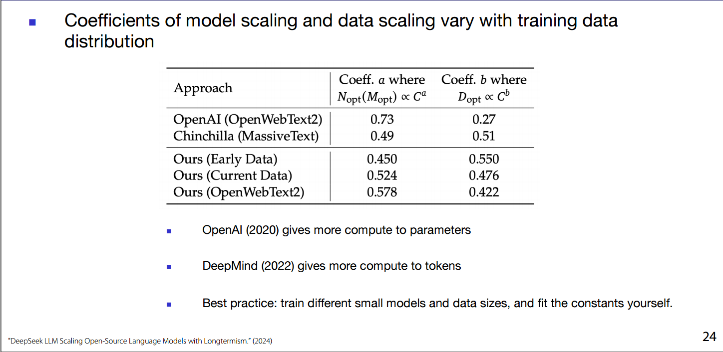
- OpenAI (2020) gives more to parameters.
- DeepMind(2022) gives more compute to tokens.
- Best practice: Train different small models of your desired architecture on different data sizes and fit the constant yourself.
- pick the lowest test loss and draw the line fitting the lowest (fit the lowest loss).
- Coefficients of model scaling and data scaling vary with the data distribution of the dataset itself.
- Wiser Compute allocation is always better than scaling-up:
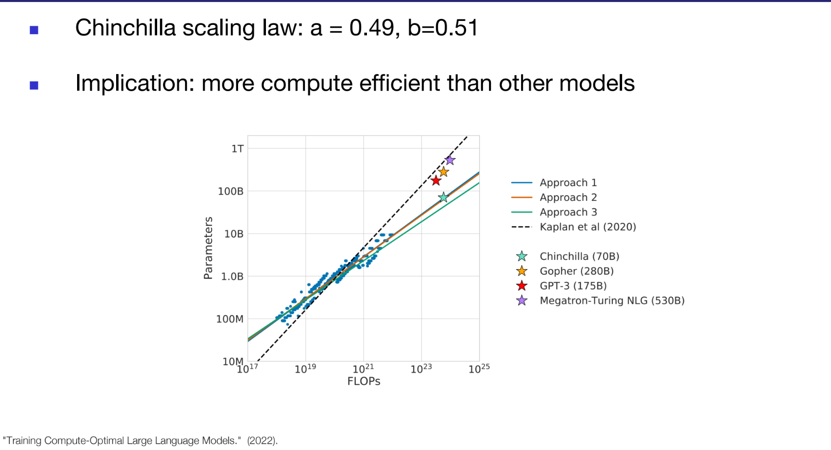
- Chinchilla outperforms Megatron by allocating compute better.
- Chinchilla law (hypothesis): a=0.49, b=0.51.
- Chinchilla (70B) model more compute efficient than:
- GPT-3(175B), Gopher(280B) and Megatron-Turing NLG (530B)
- Chinchilla has simple guidelines they created a sample suggestions table
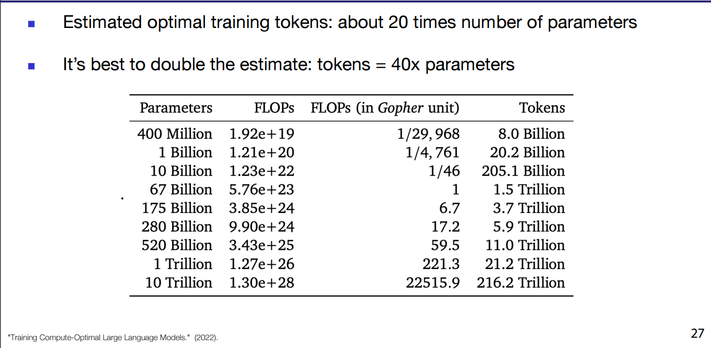
- Where FLOPs are Floating Point Operations Per Second.
- It’s better to do more than double of that proven nowadays more than 40x parameters.
- Llama 7b is trained on 7x Chinchilla optimal estimate.
- Model size can change in increasing hidden layers or number of blocks/layers or both.
-
Scaling Hypotheses are for guidance on how to spend compute more efficiently.
-
But dataset quality improvements always guarantee model improvements generally.
-
- However, Llama-3 Using 15T tokens on 8B, 70B parameters model made the performance improvements clear and as announced the models weren’t hitting saturation / convergence and 8B model great performance on various benchmarks, with Llam3-8B doing better than Llama2-70B in some cases.
- The focus on both optimizing compute and FLOPs while increasing quality of training Token Count, where 15T didn’t even saturate a 8B parameters model, will be the focus of upcoming foundational models development and research.
- Loss determines the final estimate of downstream performance, regardless of model size if they have same loss they’ll have the same performance.
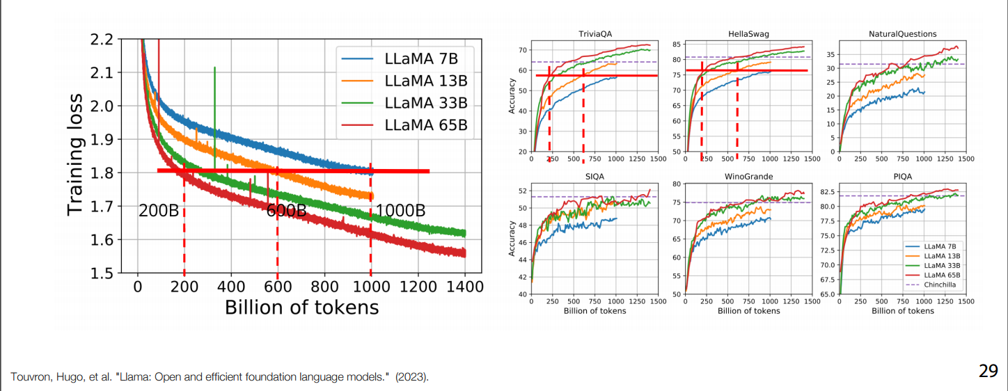
- In practice, loss can help you determine if you can go smaller.
LLM-Bottlenecks
Large Context
- Transformers cannot by default fit complex, long sequences, because Transformer attention has high memory cause.
- Example needs: Agents, World Modeling, Codebases, Genome and hyperlinked web.
- Attention weight matrix has quadratic memory cost,
- Some efforts tried to fix that for example:
- re-ordering compute as Blockwise parallel transformers as an example.
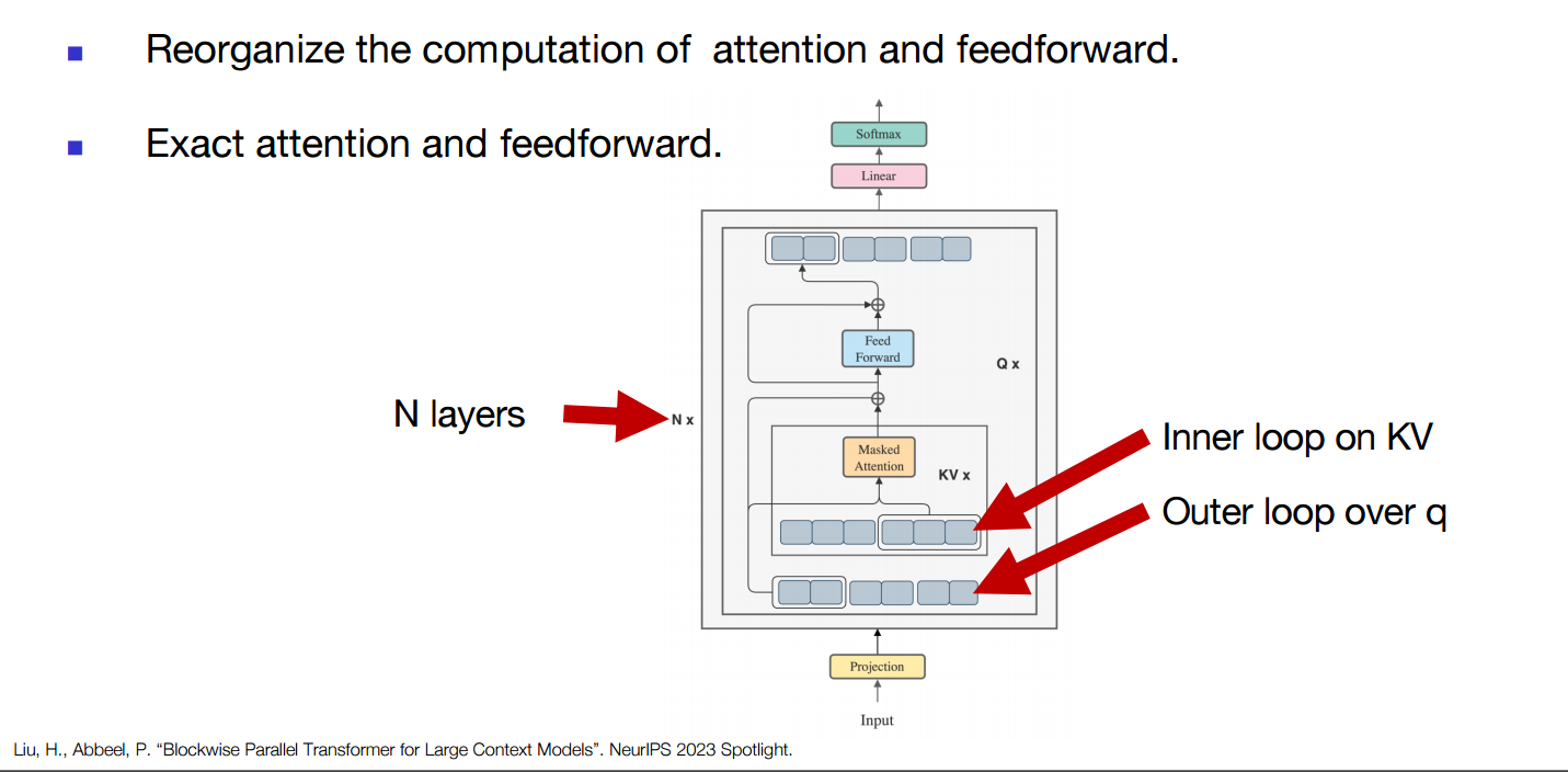
- re-ordering compute as Blockwise parallel transformers as an example.
- Standard Attention + Standard FFN (Feed-forward network): - >
- Peak of attention:
- Peak of FFN:
- Memory Efficient Attention + Standard FFN: - > (Flash Attention)
- Peak of attention:
- Peak of FFM:
- BPT: - > (Blockwise Parallel transformer)
- Peak of attention:
- Peak of FFN: , because
- 4x smaller peak activation memory
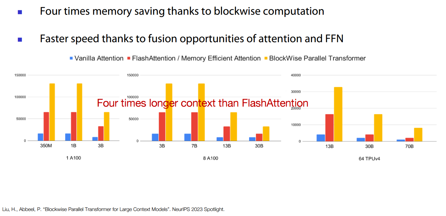
- Some efforts tried to fix that for example:
- Google tried it on Gemma models got:
- 16x expanded MLP hidden dimension.
- BPT allows 16x memory saving without overhead.
- longer sequence hence longer contexts.
- We still can’t do Million-length sequence:
- Memory cost scales with sequence length .
- chip memory have scaling limitations (we’re already pushing against physics limitations)
- Multiple GPUs in parallel for same sequence isn’t the answer as attention requires pairwise interactions.
Resources:
- Lecture 8 video : Lecture 8.
- DUL Berkeley Spring 2024 offering
- Screenshots from the Lecture 8 PDF.
- Llama 3